Question
- Between / within?
Advantages
- Adding a temporal dimension, increases number of observations → goal: inference from sample to population → sample gets closer to population due to the larger size
- Allows to analyse dynamic processes (≠ static models)
- Control for unit heterogeneity (unit = object of study, e.g. individuals, parties, countries): States are different from another, non-observable differences → omitted variable bias (not accounting for a factor that impacts both the dependent / independent variable) → this type of data can reduce the problem
- Allows multilevel / hierarchical analysis
- Because data varies not only units but also across times, helps to reduce the problem of multicollinearity
Modeling techniques for continous dependent variables
Pooled OLS Estimation
Based on the (strong) assumption that all observations are independent over time (e.g. the military spending of US in 1960 is independent from its spending in 1965) → rather unrealistic
Difference from a “normal” OLS:
Pooled OLS model:
- : constant that doesn’t vary over observations or time
- : coefficient does also not vary over observations over time (i.e. they are also constant)
- : Error unique for observation and time points
Advantages:
- increases the sample size (by adding different time points instead of looking at a cross-section only → including variation, which is good)
- allows to model period-specific effects by adding a time-dummy (by adding a variable which is 0 for all other time points except one, where it takes the value 1)
Disadvantages:
- does not control for differences within observations (unit heterogeneity) → leads to bias
- unit-specific factors correlate with one or more independent variables, estimates are biased (omitted variable bias) Violation of OLS assumption!
Solution: Control for unit hetereogeneity → error-components model
Unit heterogeneity means that units (countries, states, etc.) differ in ways not explained by observed independent variables. In other words, potentially important local factors are unobservable to the researcher” (Wilson/Butler 2007, p. 104).
Error-Components Model
Imagining that the context of observations can be captured by a variable.
Including an unobserved “context variable” → part of the error term
- If correlated with independent variable → bias (see above) → need to eliminate the effect of the variable
Assumption of the Error-Components Model: Context differs between countries but is constant over time (varies for each observation) → moves it into the error
Essentially, you’re separating the variation within a unit over time () from variation between units ().
New error term
- = constant unit-specific error (capturing the unit heterogeneity)
- This absorbds all unobserved factors that are specific to a unit and do not change over time
- = Idiosyncratic error
This also removes the constant from the overall regression equation – each observation gets its own constant ( is replaced by ) → unit specific error
This can be expanded by including time effects (varying over time, but not over observations, e.g. changes in the global economy)
So in other words:
- is something special about that observation (e.g. country)
- is something special about that specific time-point
- is the random stochastic error
Different means of controling for the temporal variation:
1. First-Difference Estimator
Removes unit-specific effects by first-differencing. This is basically an OLS model with the time-differences as variables (instead of their level).
“How does the change in for the same unit between periods explain the change in for that unit?”
What is first-differencing? Looking at differences / changes of the (in)dependent variables between time-points.
First-Difference Estimator:
- is still constant over time and space
- the part → change in the dependent variable for unit over time
- the part → change in the independent variable for unit over time
- the unit specific effect drops out automatically because it doesn’t change over time
The model estimates the effect of changes within units over time. Variables that are time-constant for a unit cannot be estimated because they are differenced away—their change is zero.
2. Fixed Effects Estimator
Fixed effects essentially compare each unit to itself over time (i.e. to their mean = most typical value).
Measures all observations in deviations of the individual time average (for example the average of the military spending of a country over all-time points).
- Also eliminates the unit specific effect because everything that is constant for a unit is part of the “baseline” which is subtracted out.
Difference between FD and FE
- FD uses consecutive differences → looks at the change between two periods
- FE uses demeaning → uses all periods simulteaneously = more efficient
- Both eliminate but in slightly different ways
Alternative: Unit-specific dummies
Less inefficient, because a lot of additional variables have to be included and estimated. It would however, produce identital estimates as the fixed effects (time-demeaned approach) (bad Adjusted R² as well)
F-Test for fixed effects
- : No unit-specific fixed effects → pooled OLS is appopriate
- : There are unit-specific effects → not appropriate → FE model is better
The R command for the F-Test compares two models:
plm::pFTest(fe_model, PooledOLS)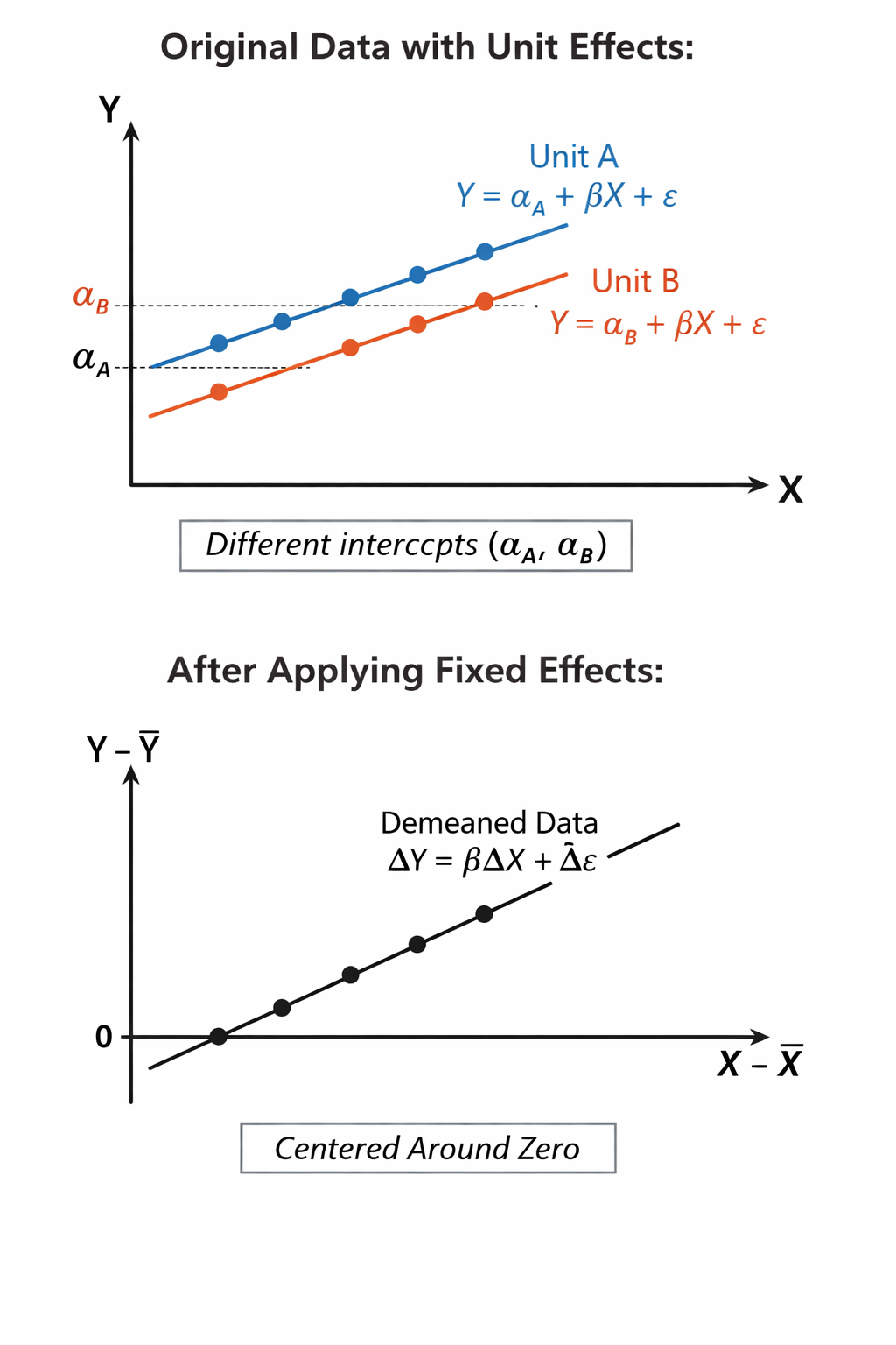
3. Random Effects Estimator
Contrary to the fixed effects estimator, here the unit effects are assumed to be random. So, can take any value. This requires the assumption that is not correlated with (otherwise the OLS assumptions would be violated).
To estimate random effects with OLS the following transformation is needed:
where:
Formula with sqrt: How much of the variation (standard deviation) is due to the stochastic error / randomness → proportion which is due to randomness
- varies between 0 and 1
- If it is very small → very close to 1 → random effect identical to the fixed effect estimator
- If it is very large → very close to 0 → identital to Pooled OLS estimator
Advantage of random effects estimator: Allows us to include time invariant variables (or ones that vary very slightly over time)
Test for random effects
- Breusch-Pagan Lagrange-Multiplier-Test
- : no random effects → Pooled OLS model works
- : random effects → RE model better
plmtest(re,model, type="bp")Tests for fixed vs. random effects
- Hausman-Wu test if some unobserved, time-invariant characteristics of the unit () are correlated with your independent variables
- : → Random and Fixed Effects should be similar
- : → Fixed Effects should be used
Possible violations of OLS model assumptions with Panel Data
There are a number of possible violations of the OLS assumptions regarding
Dynamic Panel (time series cross-sectional data) models
Auto-regressive distributed lag model
Static model:
Lagged dependent variable (LDV) model:
The dynamic models include a lagged dependent variable (LDV) as independent variable → means that current values of the dependent variable are affected by past values (e.g. path dependence)
The lagged variable is .
Autoregressive distributed lag (ARDL) model:
Includes a lag on independent variables. This is relevant is we suspect reverse causality or simultaneity. The lagged variables here are and . Allows to model dynamic processes and causal relationships.
Overview: How to choose the right model?
| yes ✅ | no ❌ | |
|---|---|---|
| Are repeated observation of the same unit of analysis legitimate observations? | → panel data | → cross-sectional data |
| Can all observations be treated as independent? | → pooled OLS | → one of the error-component models |
| Do previous periods impact current realizations of the dependent variable ? | → dynamic model | → static model |
| Are any assumptions for the error term violated? | → correct for violations in error-term or respecify the model | → estimate the model |
Binary variables
Application in R
Dataset
The dataset contains data from a number of countries over different time points, including the country’s military spending (logharitmised), their democracy score, etc.
Military expenditure is used a dependent variable
What gives the dataset a panel structure?
- multiple countries
- multiple time points
Task 1: Structure of panel dataset
Preparation: Declare the data as panel data
plm package; Create a new dataframe called Nordhaus.p
Nordhausis the source dataindexindicates which variable give the data its panel structure
Nordhaus.p <- plm::pdata.frame(Nordhaus, index = c("STATE", "YEAR"))Unbalanced panel data: Some countries don’t have data for every time point (mostly because the countries didn’t exist yet at earlier time points). Year of ranges Missing observations at some timepoint
Balanced panel: Each observation has data for each time point
plm::pdim(Nordhaus.p)Creating a plot shows the variation of different countries over time
Two sources of variation of the dependent variable:
- Within variation: Same country changes its military spending over time
- Between variation: Differences in military spending between countries at a single point
- Within + between: combination of the two (between countries and over time)
Further preparation:
Remove missing data points (necessary or just to show the number of observations??)
Calculate overall, between and within variance of the dependent variable using the function xtsum
Interpretation of the table:
- SDs: High difference between countries (some countries with very high military spending like the US, some with rather low spending), changes within countries are relatively small (the overall level within countries remain more or less the same)
2. Analysing panel data
Effect of the military spending of other countries (friends, foes) on a country’s military spending
Hint
Log variables → can be interpreted in percent
Pooled OLS Regression
lm package possible, too but here plm is used.
PooledOLS <- plm(LMILEX ~ LNFOES + LNFRIENDS + LNRGDP + DEMOC, data=Nordhaus.p, model="pooling")Output:
at the top: Information about the panel,
n: Number of countriesT: Range of time points per countryN: Number of total observations (country-years)
Sum of squares (total) - residual (unexplained) = explained sum of squares R² explains the overall variation (analog normal OLS)
Both variables are logharitmised → Changes can be interpreted in percent
LNFOES: On average a 1% increase in military spending of enemies is expected to raise a states military spending by 0.22 %.
First-difference
Includes the function diff for all of the variables which estimates the differences
FirstDiff <- plm(diff(LMILEX) ~ diff(LNFOES) + diff(LNFRIENDS) + diff(LNRGDP) + diff(DEMOC), data = Nordhaus.p, model="pooling")Output:
Interpretation:
As we only difference two values in t and t-1, we do not change the units of the variables. ⇒ A 1 percent increase in foes’ military expenditures corresponds to a 0.132 percent increase in a state’s own military spending, c.p.
Compared to the model before the direction of the effect did not change, but its size is different.
Interpretation R²
Fixed-effects model
fe_model <- plm(LMILEX ~ LNFOES + LNFRIENDS + LNRGDP + DEMOC, data=Nordhaus.p, model="within")Compared to the previous models, the coefficient for friends changed its direction
Output / Interpretation
R² : The R-squared shown in the Output gives us the total share of variation “within” the countries/“units” the model explains, i.e. the share of the variation we find between observed values of one specific country, not taking variation between countries into account.
Does not take variation between countries into account
Execute an F-Test
pFtest(fe_model, PooledOLS)Output + Interpretation
Between-estimation
Contrary to models above, this type of model tries to explain the differences in military expenditure between countries.
between <- plm(LMILEX ~ LNFOES + LNFRIENDS + LNRGDP + DEMOC,
               data=Nordhaus.p, model="between")
Random-Effects Models
re_model <- plm(LMILEX ~ LNFOES + LNFRIENDS + LNRGDP + DEMOC, data=Nordhaus.p, model="random")Specific block in the output called Effects
idiosyncratic error (randomness) + individual (country-specific), also allows for interpretation of theta
High values → close to pooled (?) effects
Interpretation: