Network Analysis

Missing

• Triad census
• Overview centrality measures

Network analysis looks at a set of actors and the relationships between them. The goal can either to describe the network (e.g. how relationships are structured) or to find explanation based on the network structure (e.g. what causes the relationships between actors or what effects do these relationships have).

Example of networks

• The members of a company forming an informal (friendships, advice-seeking) and formal (official hierarchy) network
• Nation states forming a network of trade or conflict relation

Basic terms and concepts

Term	Explanation
Nodes	The actors in a network (e.g. individuals, states, etc.)
Ties	The relationship between the actors. Depending on the type of relationship ties are also called line, link, edge or arc.
Directed vs. undirected relationships	Some relationships between actors have a direction while others have not (e.g. mutual defense alliances like NATO where each member has to help each other vs. foreign aid flows that only go in one direction) Undirected ties are called edge, directed ties are cald arc.
Binary vs. valued relationships	Some relationships are binary (yes / no) while others have a certain value or strenghts (think EU membership vs. trade volume between countries)
Dyad / Triad	A pair of two / three nodes and their relationship (regardless of whether there is a tie between them or not)

Adjacency Matrices

An adjacency matrix contains the information about the relationships (links, ties) between actors. The number of rows and columns equals to the number of actors (or nodes) in the networks $g$

Depending on the type of relationships there are different types of matrices:

Matrix	Type of relationship
Binary vs. valued adjacency matrix	Binary vs. valued relationships → $x_{ij}$ takes either values of 0 / 1 or some other numerical
Symmetrical vs. asymmetrical adjacency	Undirected vs. directed relationships → the values in the matrix are symmetrical along the diagonal ($x_{21}=x_{12}$, etc.) or not

$$X=X_{g,g}=\left[\begin{array}{cccc}{x}_{11}& x_{12}& \cdots & x_{1g}\\ x_{21}& x_{22}& \cdots & x_{2g}\\ ⋮& ⋮& x_{ij}& ⋮\\ x_{g1}& x_{g2}& \cdots & x_{gg}\end{array}\right]$$

For undirected relationships the cell values are symmetric along the main diagonal of the matrix.

For directed relationships the rows indicate the ties from senders to receivers and the columns indicate the ties from receivers to senders.

Warning

Actors are not allowed to have loops (a relationship with themselves), therefore values of $x_{11}$, $x_{22}$, etc. are always $0$.

Values within the adjacency matrix

Value	Meaning
0	no tie between actors
1	tie between actors (actors are adjacent)
$x$	strength of the tie (some numerical value, i.e. the value of traded goods between countries in USD)

Example

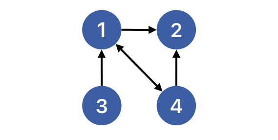
The matrix shows a network with four actors.

$$X=X_{g,g}=\left(\begin{array}{cccc}0& 1& 0& 1\\ 0& 0& 0& 0\\ 1& 0& 0& 0\\ 1& 1& 0& 0\end{array}\right)$$

To check whether it is directed or undirected we have to look at the (a)symmetry of the matrix. The relationship from actor 1 to actor 2 (seen in the second column of the first line) is 1. The reverse relationship from actor 2 to actor 1 (seen in the first column of the second line) is 0. This means that the matrix is asymmetrical and that the network is directed.

Visualised, the network looks like this:

Density

The density of a network is the share of existing ties among all potential ties in the network. So we need to find out how many ties there actually are ($L$) and how many there could be. The calculation is slightly different between directed and undirected networks.

Undirected networks

The maximum number of ties in a network with a number of $g$ nodes is:

$$g(g-1)/2$$

Because ties can’t be connected to themselves, one is subtracted. Because the network is undirected, a connection between two nodes counts as a tie regardless of its direction so the number of ties is divided by two.

The density of an undirected network is then the number of $L$ ties that exist in the network in proportion to the maximum number of ties:

$$\frac{L}{g(g-1)/2}=\frac{L\ast 2}{g(g-1)}$$

The density is 0 when L = 0 and 1 when all possible connections in the network are realised.

Directed networks

For directed networks, the principle is the same, but because a tie between two nodes can go either way, the division by two is not necessary.

The number of possible ties then is:

$$g(g-1)$$

And the density is:

$$\frac{L}{g(g-1)}$$

Once again, the values of the density can range from 0 to 1, representing everything from no connections at all to all possible ties existing and being reciprocal.

Diad / triad census

Categorises all the dyads (or triads) in a network into three diferent states:

• M = mutual
• A = asymmetric
• N = null
• X (only in triads) → look at asymmetric edges
  • D = down (edges flow in a hierarchical or linear direction)
  • U = up (edges flow opposite to some focal node)
  • C = cyclical (edges form a closed loop among three nodes)
  • T = transitive

Centrality Measures

Overview:

Centrality Measure
Degree Centrality
Betweenness Centrality
Closeness Centrality

1. Degree Centrality

The degree of a node describes the number of connections it has to other nodes. Indegree and outdegree only matter for directed networks.

Hint

• Degree refers to the raw count of connections
• Degree centrality usually refers to the normalised measured which allows for comparison across networks (but this wasn’t made really explicit in the materials)

	Definition	Calculation from matrix	Example
Degree	Number of direct connections a node has	Sum down row or column	In a network of bilateral trade agreements, if Germany has trade agreements with France, Italy, and Poland, Germany’s degree = 3.
Outdegree	Number of ties sent by a node (outgoing connections)	Sum across row	If the USA sends foreign aid to 15 countries, USA’s outdegree = 15.
Indegree	Number of ties received by a node (incoming connections)	Sum across clolumn	If Kenya receives foreign aid from 8 donor countries, Kenya’s indegree = 8.

More formalized, the calculation of degrees look like this:

Type of centrality	Description	Formula
Degree Centrality $C_D$	The numbers of nodes going from $i$ to $j$ or the other way around.	$C_D(n_i)={\sum }_{j=1}^g{x}_{ij}={\sum }_{j=1}^g{x}_{ji}$
Indegree Centrality $C_I$	The numbers of incoming connections (going from $j$ to $i$).	$C_I(n_i)={\sum }_{j=1}^g{x}_{ji}$
Outdegree Centrality $C_O$	The numbers incoming connections (going from $i$ to $j$).	$C_O(n_i)={\sum }_{j=1}^g{x}_{ij}$

Explanation:

• $C$ stands for centrality
• $n_i$ stands for a node $n$ in the network called $i$
• $x_{ji}$ is basically the adjacency matrix for the nodes $n_j$ and $n_i$. The sum sign indicates that all cases where a connection between $j$ and $i$ exists (marked by a 1 in the matrix) are summed up.
• The $g$ above the sum sign means that the step is repeated for all nodes $n$ from 1 to $g$. It basically sets the range for the summation so that all possible connections are checked.

Normalisation of Centrality Measures

$$C_D^{\prime }(n_i)=\frac{C_D(n_i)}{g-1}$$

To make the degrees of a node comparable between different networks, they have to be normalised. This happens by adjusting for the number of nodes $g$. Again, one is subtracted, because a node is not allowed to have a connection to itself. The normalised value can be interpreted in percent.

Example

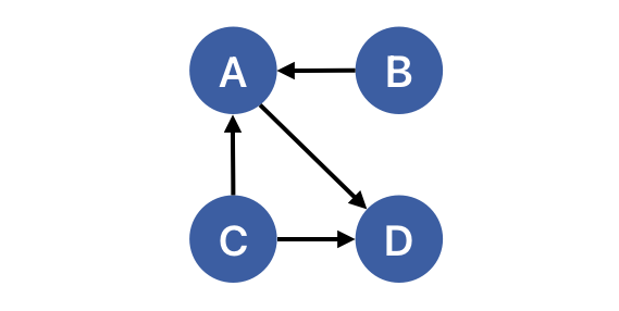
Let’s take a directed network with four nodes that have the following connections:

$B\to A,C\to A,A\to D,C\to D$

Remember that in the adjaceny matrix, the rows show the outgoing relationship from the source to the target node. The columns show the incoming connections a node has coming from other nodes.

	A	B	C	D
A	0	0	0	1
B	1	0	0	0
C	1	0	0	1
D	0	0	0	0

To calculate the indegree centrality for node A we take the values from the column A because they represent the incoming connections:

$$C_I(A)=x_{AA}+x_{BA}+x_{CA}+x_{DA}=0+1+1+0=2$$

To calculate the outdegree centrality for node B we take the values from the rows:

$$C_O(B)=x_{BA}+x_{BB}+x_{BC}+x_{BD}=1+0+0+1=2$$

To normalise the values:

$$C_I^{\prime }(A)=\frac{C_I(A)}{g-1}=\frac{2}{4-1}=\frac{2}{3}\approx 67\%$$

2. Betweenness Centrality

“Betweeness centrality […] looks at how often an actor rest between two other actors. More specifically, betweenness centrality calculates how many times an actor sits on the geodesic (i.e. the shortes path) linking to actors together” (Prell 2012, p. 104)

Steps to calculate the betweenness centrality

• Identify the geodesic(s) for each pair of actors. A geodesic is the shortest path between two nodes in a network.
• How often is the node $n_i$ part of such a geodesic?

Formula:

$$C_B(n_i)=\sum _{j<k}^i\frac{g_{j,k}(n_i)}{g_{j,k}}$$

The betweenness centrality $C_B$ for actor $n_i$

• $g_{j,k}(n_i)$: the number of geodesics from $j$ to $k$ where $n_i$ is included, divided by
• $g_{j,k}$: the number of all geodesics from $j$ to $k$
• summed up over all pairs of other nodes

Example

In this network there are two geodesics for the pair of actors $j$ and $k$, both with a length of three.

• $j\to i\to g\to k$
• $j\to f\to g\to k$

So to calculate the betweenness centrality of $i$, we would count the first geodesic in the numerator of the fraction above and the second in the denominator. To continue, we would have to do the same for all other combinations of nodes and then sum up the result.

Normalised betweenness centrality

$$C_B^{\prime }(n_i)=\frac{C_B(n_i)}{(g-1)(g-2)/2}$$

To normalise the betweenness centrality of an actor it needs to be divided through the maximally possible betweenness of a network of a size $g$. This corresponds to the maximum number of node pairs that don’t involve $i$.

Interpretation: A normalised betweenness centrality of 0 would mean that the actor is never part of any geodesic between other pairs. A value of 1 would mean that it is part of all geodesics (i.e. the center point in an undirected star network)

3. Closeness Centrality

Closeness is measured ”as the distance between actors, where actors who have the shortest distance to other actors are seen as having the most closeness centrality” (Prell 2012, p. 107)

The closeness centrality of an actor $n_i$ is 1 divided by the sum of the shortest path to each of the other nodes. The denominator by itself indicates farness which would be less intuitive, because higher values would mean less centrality.

$$C_C(n_i)=\frac{1}{{\sum }_{j=1}^{g}d(n_i,n_j)}$$

If you are, however, interested in the farness $F$, you can just keep the part in the denominator.

To normalise the closeness centrality one adjusts for the maximum value of closeness centrality which is determined by the number of actors $g$.

$$C_C(n_i)=\frac{g-1}{{\sum }_{j=1}^{g}d(n_i,n_j)}$$

Warning

Determing the closeness centrality works for connected graphs, because if some of the nodes are not connected to the rest of the network, their closeness is zero, which makes the values of $C$ really small.

Example

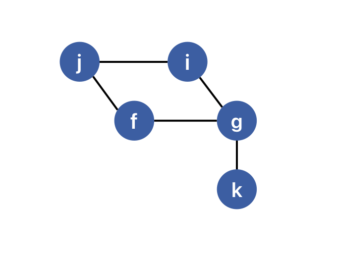
Imagine a network that looks like this:

$$A-B-C-D-E$$

To calculate the closeness centrality of $C$ we need to sum the (shortest) distances to all of the other nodes. These are:

• $d(C,A)=2$
• $d(C,B)=1$
• $d(C,D)=1$
• $d(C,E)=2$

Based on this the (normalised) closeness centrality is:

$$C_C(C)=\frac{1}{2+1+1+2}=\frac{1}{6}$$ $$C_C^{\prime }(C)=\frac{5-1}{1/6}$$

Application in R

Incomplete

1. Creating a star network and calculating indegrees

Using the package igraph, the make_star function creates a star network. The graph objects created by the package can be treated as a dataframe.

mode indicates the types of connections center indicates which node is at the center of the star network

The indegree can be calculated by using the function igraph:degree:

V(star)$indegree <- igraph::degree(star, mode = "in")
V(star)$indegree_norm <- igraph::degree(star, mode = "in", normalized = TRUE)

This also writes the calculated degrees to the star object?

Using the package intergraph, we can transform the graph object created before into a network object. This allows us to receive more information.

star_network <- intergraph::asNetwork(star)
summary(star_network)

2. Calculating indegrees, outdegrees, and density

Using the dataset transgov

In preparation, the the rows and columns are renamed to the country names (so that all cells in the matrix are just data) and transforming the object into a matrix (doesn’t change the look, but allows for other operations)

To calculate indegrees or outdegrees we can simply calculate the column or row sums of the matrix

indegrees <- colSums(matrix)
outdegrees <- c(rowSums(matrix), NA)

Optionally, both vectors can be bound to the matrix object using the rbindand cbindfunctions.

Normalisation, defining g and then performing an operation for each object.

Calculating the density can be either done manually or by transforming the matrix into an igraph object. The density can be calculated using the function edge_density.

Calculating the density by hand:

3. Calculating centrality

4. Plotting networks

5. Symmetrising networks