Factor Analysis

Missing

• Rotation
• complete R application

Similar to cluster analysis, factor analysis is a method used to identify patterns in data. The difference here is that the groups are not formed from the objects or observations in the data. Instead, single variables are grouped together.

This for example allows us to:

• simplify the data structure by reducing a large number of observed variables to a smaller set of underlying factors
• identify hidden patterns in how variables correlate with each other and uncover latent, underlying dimensions
• create indicators for theoretical constructs

There are two different methods of factor analysis who have slightly different assumptions. The basic idea is, however, to create a correlation matrix of all variables and then group them into a number of (previously determined) factors.

Cluster vs. factor analysis

• Cluster analysis groups objects / cases based on similarities (similar values on a set of variables)
• Factor analysis groups variables based on their correlations

Overview over the two different methods

	Principal Components Analysis	Factor Analysis
Variance	completly covered by the factors	Common vs. unique variance
Model assumptions	No error / unique factors	Includes unique factors
Communality	Always = 1 (all factors are extracted)	Always < 1
Uniqueness	Always = 0	Always > 0
When to use?	For reducing data into a lower number of dimensions	To find out about underlying latent variables

Principal Components Analysis (PCA)

Formula:

$x_{ik}=a_{k1}\ast p_{i1}+a_{k2}\ast p_{i2}+...+a_{kq}\ast p_{iq}$

• $x_{ik}$: The observed value of unit $i$ on variable $k$
• $a_{kq}$: Factor Loading of variable k on factor $q$
• $p_{iq}$: Factor score of unit i on factor q

Factor Analysis

Factor analysis assumes that not all of the variance in the data can be traced back to the common factors but that some of it is due other influences (e.g. measurement errors)

Formula:

$x_{ik}=a_{k1}\ast p_{i1}+a_{k2}\ast p_{i2}+...+a_{kq}\ast p_{iq}+w_k\ast u_{ik}$

The formula is the same as for PCA except the last product ($w_k\ast u_{ik}$) which represents the variance which is not accounted for by the common factors.

Relevant concepts

Concept	Description
Factor Loadings	Correlation between a single variable and a factor.
Factor Scores	A specific value a specific observation has on a factor (one score per factor per observation)
Eigenvalue	Amount of variance explained by a single factor across all variables.
Communality	The variance of a single variable accounted for by all the factors.
Uniqueness	The variance of a single variable not accounted for by all the factors.

Hint

• Factor loadings are used to interpret the factors (what variables form a factor together).
• Factor scores show how much of a factor applies to each observation.

Factor loading

The factor loading describes the relationship between a (observed) variable variable $k$ and the (unobserved) factor $q$. They are properties of the variables, not the observations.

Meaning: Loadings tell you what the factor represents: A high factor loading means that the variable is strongly associated with, or well represented by, the factor.

Value range: Factor loadings can take values from -1 to 1 (as they are essentially correlations betwen variables and a factor).

In principal component analysis (for z-standardized variables and as long as no skewed rotation was performed), the factor loadings indicate the correlation between a certain variable k and a certain extracted factor.

Squared factor loadings: When the factor loading is squared it indicates the variance of a single variable that is explained by the factor (similarly to the sums of squares in OLS).

Example

Variable	Factor 1 Loading	Squared Loading	Explained variance
Math	0.7	0.49	49%
Science	0.8	0.64	64%
English	0.3	0.09	9%

Interpretation:

• Science loads 0.8 and is strongly related to factor 1
• Science loads 0.3 and is weakly related to factor 1

Factor score

The factor score is the estimated score each observation has on one of the factors (i.e. the value of the factor for each case). They are properties of the observations, not of the variables.

Eigenvalue

The Eigenvalue indicates the total variance explained by a factor. It consists of the sum of the squared factor loadings of all variables for a single factor.

$${\lambda }_q=\sum _{k=1}^K=a_{kq}^2$$

• $K$ = Number of variables
• ${\lambda }_q$ = Eigenvalue of factor $q$
• $a_{kq}$ = Factor loading of variable $k$ on factor $q$

Because the squared factor loading of each variable can range from 0 to 1, the maximum possible Eigenvalue of each factor corresponds to the number of variables.

Example

The factor analysis contains 10 variables. The theoretical maximum Eigenvalue of any of the factors is 10. An Eigenvalue of 10 would mean that all of the variance of the variables is explained by that single factor.

Communality

The communality is the shared variance on a single variable across all factors (i.e. the sum of the squared factor loadings). IIt shows how much of the variable’s variance is accounted for by the extracted factors.

Formula:

$$h_k^2=\sum _{q=1}^Q{a}_{kq}^2$$

Reading: The communality $h^2$ of the variable $k$ consists of the squared factor loadings $a^2$ of variable $k$ which are summed up over all the individual factors $q$.

Example

Let‘s take an example variable in a factor analysis with four factors. The loadings of each factor for this specific variable are -0.07, 0.74, 0.17, and 0.08.

The calculation of the communality then looks like this:

$$h^2=(-0.07{)}^{²}+(0.74{)}^{²}+(0.17{)}^{²}+(0.08{)}^{²}=0.59$$

This means that 59 % of the variance of that variable is explained by the four factors.

Uniqueness

The uniqueness is the opposite of the communality. It indicates the share of the variance (of a single variable) that is not explained by the factors.

Formula: $u^2=1-h^2$

Rotation

Application in R

Dataset

The dataset contains observations on countries and variables on different aspects of the political system such as the number of parties, the degree of federalism and so on.

1. Preparing the dataset and creating a correlation matrix

vatter <- import("Vatter2009.dta")
 
# Data wrangling
vatter_short <- vatter %>% 
  select(-country, -year) # keep all variables except "country" and "year"
row.names(vatter_short) <- vatter$country
 
# Correlation matrix with `cor()`:
vatter_cor <- cor(vatter_short) 
vatter_cor[upper.tri(vatter_cor)]<- NA # Setting the "upper triangle" as missings for easier visual interpr
View(round(vatter_cor, digits=4))

2. Performing a Principal Component Analysis

The command principal performs a PCA. The first argument indicates the correlation table used for the analysis, nfactors indicates the number of factors we want to extract. Here we assume 4 underlying factors. rotation is not applied.

pca_results <- psych::principal(cor(vatter_short), 
                                nfactors=4, 
                                rotate="none")
pca_results

Output (split in two):

Principal Components Analysis
Call: psych::principal(r = cor(vatter_short), nfactors = 4, rotate = "none")
Standardized loadings (pattern matrix) based upon correlation matrix
               PC1   PC2   PC3   PC4   h2   u2 com
effparties   -0.07  0.74  0.17  0.08 0.59 0.41 1.2
execleg       0.25  0.73 -0.23 -0.10 0.66 0.34 1.5
disprop       0.09 -0.76  0.31  0.31 0.78 0.22 1.7
interest     -0.41  0.67 -0.31  0.22 0.76 0.24 2.4
centralbank  -0.48  0.51  0.02  0.56 0.80 0.20 2.9
federal       0.88  0.10 -0.04  0.08 0.80 0.20 1.0
taxes         0.70  0.26  0.05 -0.44 0.76 0.24 2.0
bicam         0.83 -0.03  0.24  0.34 0.86 0.14 1.5
constitution  0.66  0.33 -0.25 -0.09 0.61 0.39 1.8
judreview     0.65  0.04 -0.09  0.52 0.71 0.29 2.0
cabinets     -0.17  0.41  0.73 -0.18 0.75 0.25 1.8
directdem     0.09  0.36  0.75  0.04 0.70 0.30 1.5
 
                       PC1  PC2  PC3  PC4
SS loadings           3.33 2.85 1.50 1.10
Proportion Var        0.28 0.24 0.13 0.09
Cumulative Var        0.28 0.52 0.64 0.73
Proportion Explained  0.38 0.32 0.17 0.13
Cumulative Proportion 0.38 0.70 0.87 1.00
 
Mean item complexity =  1.8
Test of the hypothesis that 4 components are sufficient.
 
The root mean square of the residuals (RMSR) is  0.09 
 
Fit based upon off diagonal values = 0.92

The first part of the output shows the factor loadings for each variable (lines) + each factor (columns)

• E.g. for the variable effparties the second factor (0.74) can explain a high share of the variance in the variable. To calculate the exact variance the factor loading can be squared
• u2 shows the Uniqueness
• h2 shows the Communality
• com shows complexity (not covered here)

The second part shows information on the factors

• SS loading shows the Eigenvalues
• Proportion Var shows the proportional variance explained by one factor = Eigenvalues (or SS loading divided by the number of variables
• Cumulative Var shows an ongoing addition of the proportional variances from one to another (would go up to 1)

The results can only be display partially using the following commands:

pca_results$loadings
pca_results$uniquenesses

3. Creating a scree plot

psych::VSS.scree(cor(vatter_short), 
                 main="Scree plot of eigenvalues by factor")
abline(1,0, col="red")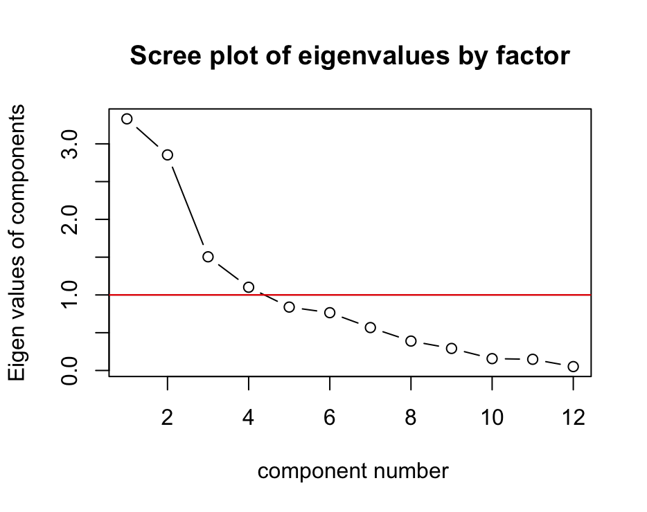

Interpretation:

• The y-axis shows the eigenvalues of components.
• The x-axis shows number of components.
• The line shows how the eigenvalues drop with an increasing number of components.

According to the Kaiser-Criterion (a rule of thumbs which says to retain factors with eigenvalues that are greater that one should be extracted), the plot shows that four factors should be extracted.

4. Rotation

Goal: Maximising the variance explained by the factors and make sure that each variable only fits to one factor (to the extent possible)

pca_results_rotated <- psych::principal(cor(vatter_short),
                                        nfactors=3,
                                        rotate="Varimax") 
pca_results_rotated

Varimax = Orthogonal rotation (preferable) Promax = Oblique rotation

round(pca_results_rotated$rot.mat, digits=4)

Rotation matrix:

        [,1]    [,2]    [,3]
[1,]  0.9862 -0.1568 -0.0525
[2,]  0.1647  0.9036  0.3954
[3,] -0.0145 -0.3986  0.9170

4. Predicting and interpreting factor scores

factor_scores <- predict(pca_results,vatter_short)

			 PC1         PC2          PC3
Australia    1.56317761 -1.15042788  0.265304376
Austria      0.22205895  0.40163084 -0.752673621
[...]
UK          -0.57633764 -2.35926295  0.170078988
USA          2.03517192 -0.38503274 -1.080843363