Cluster Analysis

Missing

• Pseudo-F score explanation
• Last R excercise

The goal of cluster analysis is to find groups in data (i.e. to reduce the dimensionality of the data by grouping objects based on their attributes). The clusters that are created should have high within-group homoegeneity and high between-group hetereogeneity.

Example

Parties can be grouped together depending on their position on the left-right spectrum

Cluster analysis can be used to either exploratively generate groups based on the underlying data or to test theoretically based groupings.

Steps

1. Selecting objects and variables

• Variables form a multi-dimensional feature space (like a coordinate grid)
• Depending on the variable values, each object has a specific position on this space (point in the grid)
• The results of the cluster analysis depend on the chosen variables

2. Selecting a similarity / dissimilarity measure

Which type of measure to chose?

• Nominal / binary variables → association measures
• Metric variables → distance measures

Warning

The same data can lead to different clustering results depending on the (dis)similarity measure one choses.

Similarity measures for binary variables

The base idea is to compare each pair of objects and see how they relate on each variable:

We look at two objects at a time and compare their traits (i.e. their variables). Since every trait is binary (either “yes” or “no”), there are only four possible ways a pair can match up. We simply count how many times each match happens.

Observations j (columns) and i (rows)	yes	no
yes	$a$ (i = yes, j = yes)	$b$ (i = yes, j = no)
no	$c$ (i = no, j = yes)	$d$ (i = no, j = no)

$a$ and $d$ can also be described as agreements, $b$ and $c$ can be described as disagreements.

Based on this count, a number of similarity measures can be calculated:

Similarity Measure	Formula	Description
Russel	$\frac{a}{a+b+c+d}$	Number of variables where both observations are true in relation to the total of possible combinations (including a)
Matching	$\frac{a+d}{a+b+c+d}$	Number of variables where both obervation match (both true or false) in relation to all the other possible combinations
Jaccard	$\frac{a}{a+b+c}$	Number of variables where both are true in relation to the combinations where at least one variable is true (thus ignoring cases where both are false)
Rogers	$\frac{a+d}{(a+d)+2(b+c)}$	Same as the Matching measure, but gives double the weight to cases where both observations don’t share the same value (disagree)
Dice	$\frac{2a}{2a+b+c}$	Similar to Jaccard, but doubles the weight to cases where both observations have the same attribute (agreements)

Interpretation: A higher value means a higher similarity between the two observations.

Example

We are analysing three countries over four variables.

The logic is to compare each pair individually and count the number of variables that apply to each of the four possible combinations for each variable (see above).

Variable	Germany	France	United Kingdom
EU member	1	1	0
Federal State	1	0	0
Nuclear Power	0	1	1
Presidential System	0	0	0

To then calculate, for example, the Russel index for Germany and France each of the four cases have to be counted:

• $a$ (both = yes) = 1
• $b$ (Germany = yes, France = no) = 1
• $c$ (Germany = no, France = yes) = 1
• $d$ (both = no) = 1

Calculation: $\frac{a}{a+b+c+d}=\frac{1}{1+1+1+1}=\frac{1}{4}=0.25$

The same can now be done for the other pairs: For example, the index for Germany and the UK is 0 (because the countries don’t share any variables that are both true / have the value 1). This means, that Germany is more similar to France than the UK.

Calculating dissimilarity measures

Dissimilarity measures for binary variables can be calculated by subtracting the similarity measure from 1.

Example: Jaccard similarity $=0.25$ → Jaccard dissimilartiy $=1-0.25=0.75$

Dissimilarity Measures for metric variables

In general, $d_{i,m}$ indicates the distance between the two different objects $i$ and $m$ (for example two countries). $k$ indicates one specific variable (such as GDP per capita), $K$ refers to all the variables used for the analysis.

Measure	Formula	Description
City-Block-Distance (also Manhattan Distance)	$d_{i,m}^{CITY}={\sum }_{k=1}^K|x_{ik}-x_{mk}|$	The absolute difference between the objects on a specific variable $k$ is calculated. The result is then summed up over all the different variables.
Euclidean Distance	$d_{i,m}^{EUKL}=\sqrt{{\sum }_{k=1}^K(x_{ik}-x_{mk}{)}^2}$	The underlying principle is the same, but the different variable values for the two objects are squared to avoid negative values, in case the value of the variable $k$ is larger for object $m$ than it is for object $i$. This equals the method for calculating the hypotenuse of a triangle (pythagorean theorem).
Squared Euclidean Distance	$d_{i,m}^Q={\sum }_{k=1}^K(x_{ik}-x_{mk}{)}^2$	Same as above, except the values remain squared.

Hint

The main difference between these measures is their way to deal with negative values for the difference between of the two objects. Negative values are unwanted here because all the differences between objects are summed up and should thus not decrease the sum just because the value of the second variable happens to be larger than that of the first.

3. Transforming / standardising the data

This is relevant for metric variables. In some cases it can be necessary to standardise their values, because variables that have a much larger range than others can skew the results.

A method of standardisation is the z-score standardisation:

$$z_{ik}=\frac{x_{ik}-{\overline{x}}_k}{s_k}$$

• $z_{i}k$ is the standardized value for object $i$ on variable $k$
• $x_{ik}$ is the original value for objects $i$ on variable $k$
• ${\overline{x}}_k$ is the mean of variable $k$ across all objects
• $s_k$ = Standard deviation of variable $k$

Example

Countries are clustered along the variables “GDP per capita” and “democracy score”.

Because the first can reach values up to several thousands and the other usually remains lower than ten, the variation on the second variable doesn’t really make a difference when calculating the distance on which the dissimilarity measures are based.

Country	GDP (billions €)	Democracy Score (0-10)
Germany	3,800	8
France	2,600	9
Denmark	350	10
We could calculate the Euclidean distance without standardisation:

$$\sqrt{(3800-2600{)}^2+(8-9{)}^2}=\sqrt{1440000-1}\approx 1200$$

We see that the difference between the countries’ GDP completly outsizes any difference in their democracy score. This means that the clustering would almost entirely on GDP, and democracy scores would be ignored.

To solve this, we need to standardise. To do this we first calculate the mean value, then the standard deviation for both variables and then calculate the scores for each country and variable using the respective values.

The result is:

Country	GDP (z-score)	Democracy (z-score)
Germany	1.08	-0.71
France	0.24	0.71
Denmark	-1.33	1.00

The interpretation is:

• $z=1.08$ (Germany’s GDP): This GDP is 1.08 standard deviations abovethe average
• $z=0.24$ (France’s GDP): This GDP is 0.24 standard deviations above the average
• $z=-1.33$ (Denmark’s GDP): This GDP is 1.33 standard deviations below the average
• $z=0$: Exactly at the mean
• Positive $z$: Above average
• Negative $z$: Below average

4. Selecting a clustering procedure

Hierarchical clustering solutions

Method	Starting point
Agglomerative Methods	Each individual object forms a single cluster
Divisive Methods	All objects form a single cluster

Agglomerative Algorithm

1. Starting point: Each object forms a single cluster. At this point the number of clusters equals the number of objects $N$.
2. For each pair, a (dis)similarity measure is calculated. On this basis a distance / similarity matrix is created.
3. The pair with the highest (or smallest) similarity is identified and combined into a new cluster. This leads to a reduction of the number of clusters by 1.
4. The previous steps are repeated.

Linking Methods for multi-member clusters

What if a cluster has multiple members? There are different ways to proceed:

$D$ is the distance, the existing cluster is $A$ and the newly formed cluster is $B+C$ .

Method	Distance between new and other cluster	Effects
Single Linkage (nearest neighbour)	Shortest possible distance between cluster members $D(A;B+C)=min[D(A,B);D(A,C)]$	- Results in large, heterogenous groups (bad) - Can lead to chaining
Complete Linkage (farthest neighbour)	Maximal possible distance between cluster members $D(A;B+C)=max[D(A,B);D(A,C)]$	- Results in small, homogenous groups (good) - Can be influenced by extreme objects
Average Linkage	Average distance between cluster members	- Includes all cluster members (as opposed to the extremes) - Leads to small and equal within-cluster variation (good)
Centroid Method	Distance between cluster centroid, i.e. the mean value of all objects’ values across all variables	- Also based on all cluster members - Moving centroids (caused by changing mean values after each cluster merging) can lead to puzzling results
Ward’s method	Combination of clusters depending on the smallest increase in within-cluster sum of squares	- Results in homogenous, small groups (good) - Requires metrically scaled variables (to calculate sum of squares)

Chaining

Chaining happens when members at the extremes of each cluster are merged. This can be counterproductive as it creates cluster with members that differ greatly from another (i.e. high within-group hetereogeneity)

5. Implementing the clustering procedure

see Application in R

6. Deciding on the number of clusters to be formed

The ideal number of clusters can be determined using

• a dendogram
• the Scree-Test
• the Pseudo-F index

Dendograms

A dendogram displays how observations merge into clusters at different (dis)similarity levels.

Interpretation: You can read by visualising a horizontal line that moves from the top to the bottom. At each height the number of vertical lines that cross the imaginary line shows the number of clusters at that (dis)similarity level. A higher gap between horizontal lines means a high jump in dissimilarity.

Depending on the clustering procedure, the dendograms look different.

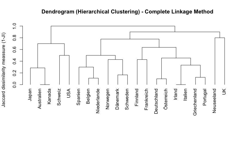
Example

In the dendogramm above Australia and Canada are very similar to each other (indicated by the minimal jump in dissimilarity). On the contrary, New Zealand and the UK are very dissimilar from each other (high jump in dissimilarity before the two lines join)

Scree plots

A scree plot shows the dissimilarity on the y-axis and the number of clusters on the x-axis. With each additional cluster the similarity increases.

This (sort of) allows us to identify the ideal number of clusters by looking for a shoulder in the graph, i.e. the point where the similarity we gain from adding an additional cluster stops being substantial.

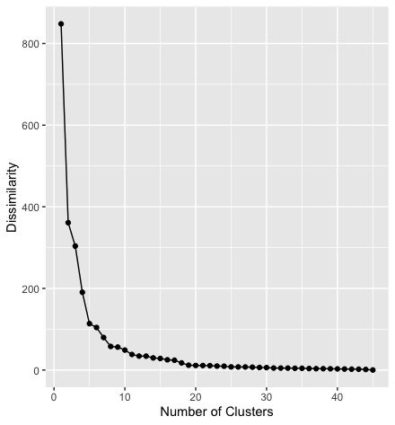
Example

In the scree plot above the step from one to two clusters reduces the dissimilarity by more than half. Adding more clusters reduces the dissimilarity further, but by decreasing amounts. From the 8th cluster on the dissimilarity is not substantially reduced by adding more clusters.

Measures of Heterogeneity / Pseudo F-Index

Formula:

$\frac{BGSS}{C-1}/\frac{WGSS}{N-C}$

• $BGSS$: Between-group sum of squares
  • The sum of squared distance between cluster centroids
• $WGSS$: Within-group sum of squares
  • The sum of squared distances between each object and other objects in the same cluster
• $N$: Number of objects
• $C$: Number of clusters in the respective step of the clustering procedure

Interpretation: A high value indicates high within-group-homoegeneity and high between-group heterogeneity. This means, one should aim to go for the number of clusters where the index’ value is the highest.

7. Interpreting + validating the clusters

Application in R

1. Calculating similarity measures for binary variables

Dataset

The dataset contains a list of countries and their characteristics in the form of binary variables, for example, whether they have a monarch or a president as head of state, if they are federally organised, member of the EU, etc.

Step 1: Preparing the data

• First, the dataset is imported into a dataframe called data.
• Then we create a new dataframe called dfand only keep a few selected variables using the select function. We also use the values of the column land to define to row names, so that the country names are not part of the actual data anymore.
• Finally, we only keep the values of the first three rows to simplify the dataset and display its contents.

data <- import("Wagschal1999.dta")
 
df <- data %>% 
  select(monarch, zweikammer, foederalismus, wahlsystem_verh, zentralbank_unabh) 
row.names(df) <- data$land
 
df <- df[1:3,]
df

The output looks like this:

Country	monarch	zweikammer	foederalismus	wahlsystem_verh	zentralbank_unabh
Australien	1	1	1	0	0
Belgien	1	1	1	1	0
Dänemark	1	0	0	1	0

Step 2: Calculating the similarity measures

The designdist command from the package vegan lets you define the dissimilarity measure you want to calculate on your own.

vegan::designdist(df, "a/(a+b+c)", abcd = TRUE)
as.matrix(designdist(df, "a/(a+b+c)", abcd = TRUE))

The arguments of the function designdist are:

• df: the data to use
• "a/(a+b+c)": the equation that should be used to calculate the dissimilarity (here the Jaccard measure is used)
• abcd = TRUE: defines that the formula follows the notation used above ($a$ for shared occurances, etc.)

The second line tells R simply wraps the function from the first line into a second function (as.matrix) which causes the results to show as a complete (i.e. mirrored) matrix.

The output then looks like this:

> vegan::designdist(df, "a/(a+b+c)", abcd = TRUE)
         Australien Belgien
Belgien        0.75        
Dänemark       0.25    0.50
 
> as.matrix(designdist(df, "a/(a+b+c)", abcd = TRUE))
           Australien Belgien Dänemark
Australien       0.00    0.75     0.25
Belgien          0.75    0.00     0.50
Dänemark         0.25    0.50     0.00

Interpretation:

Based on the included variables Australia and Belgium form the pair of countries that is the most similar to each other. This is followed by Belgium and Denmark. Australia and Denmark are the least similar to each other.

2. Performing a cluster analysis with binary data

This task uses the same dataset, but this time all the countries are included.

Step 1: Preparing the data

We keep all variable except the variable land which we use again to name the row names.

df <- data %>% 
  dplyr::select(-land) 
row.names(df) <- data$land

Step 2: Calculating the Jaccard similarity and dissimilarity

This works exactly as above, only that we calculate the dissimilarity by subtracting the similarity measure by 1. This is necessary for the following step.

jaccard_similarity  <- designdist(df, "a/(a+b+c)", abcd = TRUE)
jaccard_dissimilarity <- 1-designdist(df, "a/(a+b+c)", abcd = TRUE)
# alternatively:
jaccard_dissimilarity <- 1-jaccard_similarity

Step 3: Performing a cluster analysis using the single linkage measure

The command hclust performs a cluster analysis using the set of dissimilarities we created in the previous step. The results are stored in the object fit which is then used to plot the dendogram.

fit <- hclust(jaccard_dissimilarity, method = "single")
 
plot(fit, hang = -1, main = "Dendrogram (Hierarchical Clustering) - Single Linkage Method", ylab="Jaccard dissimilarity meassure (1-JI)",  xlab= "", sub="")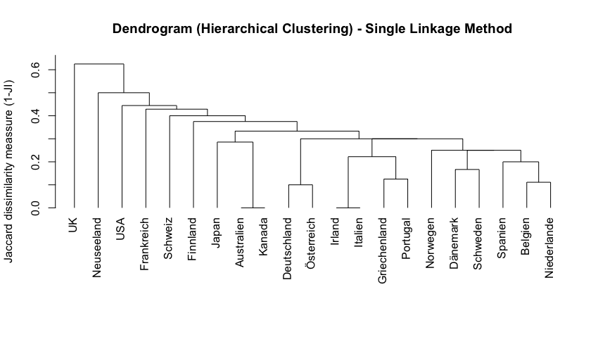

Step 4: Performing a cluster analysis using the complete linkage measure

Same principal as above, the only difference is the linkage method.

fit2 <- hclust(jaccard_dissimilarity, method = "complete")
 
plot(fit2, hang = -1, main = "Dendrogram (Hierarchical Clustering) - Complete Linkage Method", ylab="Jaccard dissimilarity meassure (1-JI)", xlab= "", sub="")

Step 4: Decide on the number of clusters

Step 5: Create a cluster variable

3. Calculating distance measures with metric-scaled data

Dataset

The dataset contains information on election districts (“Wahlkreise”) in Bavaria for the federal elections in 2013 and 2017, including variables on the number of eligble voters, vote counts for different parties, etc.

Step 1: Preparing the data

The code imports the dataset and only keeps two of the observations (“Wahlkreise) and five of the variables.

BTW <- import("BTW2017_BY.dta")
row.names(BTW) <- BTW$Gebiet
 
data_subset <- BTW %>% 
  select(Nr, Gebiet, Union2017_proz, AfD2017_proz) %>% 
  filter(Nr==229|Nr==220)

Result:

Nr	Gebiet	Union2017_proz	AfD2017_proz
229	Passau	40.54	16.06
220	München-West/Mitte	29.76	7.73

Step 2: Calculating distance measures by hand

Euclidean distance:

$$\begin{gathered} d_{i,m}^{EUKL}=\sqrt{\sum _{k=1}^K(x_{ik}-x_{mk}{)}^2} \\ =\sqrt{(40.54-29.76{)}^2+(16.06-7.73{)}^2} \\ =13.62 \end{gathered}$$

Manhattan distance:

$d_{i,m}^{CITY}={\sum }_{k=1}^K|x_{ik}-x_{mk}|=|40.54-29.76|+|16.06-7.73|=19.11$

Hint

In this example the absolute values are not really necessary because the values of the variable Union are in both cases larger than the values of the variable AfD so that there is no need to deal with negative values.

Step 3: Calculating distance measures in R

To calculate the distance measures we use the function dist. The first argument indicates that the function should only use the two columbns of the dataframe data_subset that are named Union2017_proz and AfD2017_proz.

X_L1 <- dist(data_subset[, c("Union2017_proz", "AfD2017_proz")], method = "euclidean")
print(X_L1)
 
X_L2 <- dist(data_subset[, c("Union2017_proz", "AfD2017_proz")], method = "manhattan")
print(X_L2)

Output:

> print(X_L1)
                     Passau
München-West/Mitte 13.62339
 
> print(X_L2)
                     Passau
München-West/Mitte 19.10887

4. Performing a cluster analysis with metric data

Missing