Linear Regression

Missing

• Hypothesis testing
• Omitted variable bias
• Degrees of freedom

Basic structure of linear regression models

Population regression model:

$$y_1={ß}_0+{ß}_1{x}_1+{ϵ}_i$$

This model shows the true relationship between $y$ and $x$. The equation consists of a systematic component (linear relationship) and a stochastic component ${ϵ}_i$ (error term or randomness).

Sample regression model:

$$y_1={\widehat{ß}}_0+{\widehat{ß}}_1{x}_1+{\widehat{ϵ}}_i$$

The equation consists of a estimated systematic component (the estimated regression line) and a stochastic component (residual).

• ${ß}_0$ (also often indicated as $\alpha$) = Intercept / Constant
  • (Theoretical) value of the dependent variable $y$ when $x$ is 0. Sometimes the independent variable doesn‘t reach this value in which case the value has no practical meaning
• ${ß}_1$ = Slope of the line
  • Each increase of $x$ leads to an increase of $y$ by the amount of $\beta$
  • Positive values = positive relationship where an increase in $x$ leads to an increase in $y$
  • Negative values = negative relationship where an increase in $x$ leads to a decrease in $y$
  • The unit of change depends on the unit of the dependent variable $Y$ (e.g. percentage of GDP in government spending → change in percent)
• $ϵ$ = Error term
  • The error term describes all unobserved influences on $y$ that are not caused by $x$. For this to hold, the assumption that the error term $ϵ$ is not correlated with the independent variable $x$ has to be fulfilled (see OLS assumptions)

What’s the difference between the two?

The population regression model represents the true relationship in the entire population. Because we usually can not draw a full sample of the entire population it is normally unknown and must be estimated.

Population regression model	Sample regression model
True parameters	Estimated parameters
True errors	Residuals

Estimation method: Ordinary Least Squares

The basic idea behind the ordinary least squares method is to minimise the sum of the squared residuals.

Requirements:

• Continous dependent variable
• Continous or categorical independent variables

Step-by-step:

• What are the residuals?
  • The residuals (also called error terms) are the difference between the estimation made by the model and the actual (observed) position of each point in the data.
• Why are they summed?
  • Summing combines individual errors into a single measure of total model fit. Imagine moving from a single data point to the whole regression line that we are trying to fit.
• Why are they squared?
  • Squaring the differences avoids that positive and negative deviations from the regression line cancel each other out. It also weighs larger distances of data points more strongly.

Assumptions of OLS

see OLS assumptions

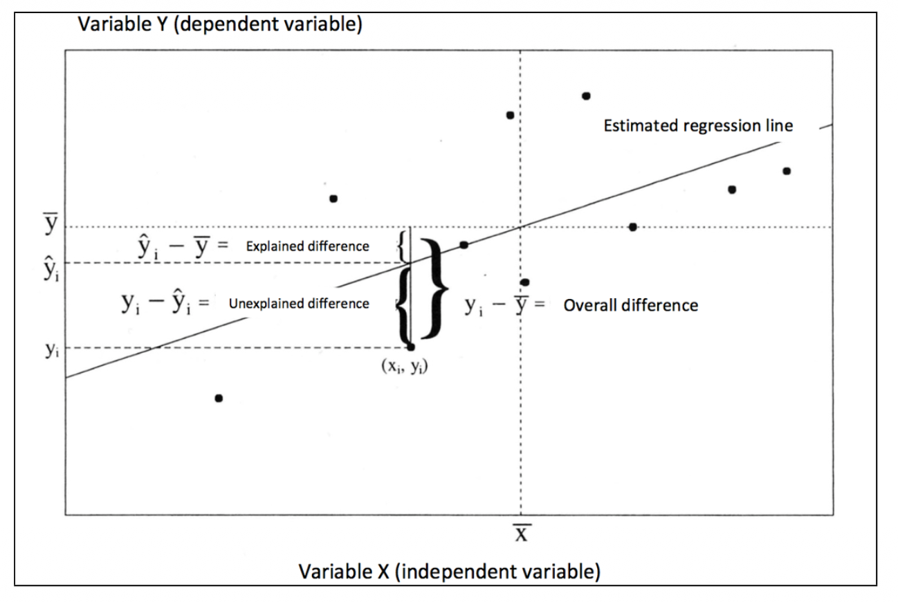
Analysis of Variance (ANOVA)

$$\sum (y_i-\overline{y}{)}^2=\sum ({\hat{y}}_i-\overline{y}{)}^2=\sum (y_i-\hat{y}{)}^2$$ $$\text{TSS}=\text{ESS}+\text{USS}$$

The variance is a statistical measure that quantifies the spread or dispersion of data points around their mean. It measures how much individual observations $y_i$ differ from the average value $\overline{y}$. Because the negative and positive differences cancel each other out each difference is quared.

The total sum of squares (overall distance) can then be separated into the the sum of explained and unexplained sum of squares:

Hypothesis testing (t-Test)

Tests the statistical significance of a single coefficient

$$T=\frac{\widehat{ß}-{ß}_{H0}}{se(\widehat{ß})}$$

Warning

The value of ${ß}_{H0}$ is (in almost every case) 0, therefore one can simply assume $T=\frac{\widehat{ß}}{se(\widehat{ß})}$

Confidence intervalls

Measures of model quality

Root Mean Square Error (MSE)

The Root Mean Square Error indicates by how many units (measured in units of y) on average the data points are away from the estimated regression line.

$\sqrt{\frac{USS}{n-K}}$

• $USS$ = Unexplained Sums of squares
• $n$ = Number of observations
• $K$ = Degrees of freedom, i.e. number of estimated parameters (intercept + independent variables)

R² / Adjusted R²

Proportion of variance explained by the model (→ see R²)

$$R^2=\frac{MSS}{TSS}$$

F-Test

The F-Test test whether the model as a whole has explanatory power. It basically asks whether the regression model is any better than just using the mean of $y$ to predict all values.

Null hypothesis $H_0$	$R^2=0$	all slope coefficients are 0 → model explains nothing
Alternative hypothesis $H_1$	$R^2>0$	at leas one coefficient is larger than 0 → model has at least some explanatory power

Formula:

$$F=\frac{ESS/(K-1)}{USS/(n-K)}=\frac{MSM}{MSE}$$

• $ESS$ = explained sums of squares
• $USS$ = unexplained sums of squares
• $K$ = number of parameters (all independent variables + intercept)
• $n$ = number of observations
• $MSM$ = Mean Square Model
• $MSE$ = Mean Square Error

Interpretation:

• Check the F-value (higher value = higher chance that the model explains something; value close to 1 = model not much better than no model at all)
• Check the p-value (value < 0.05 = model is statistically significant; value > 0.05 value is not statistically significant)

Hint

The F-test evaluates the entire model, while t-tests evaluate individual coefficients. Even if the F-test is significant, some individual coefficients might not be

Multivariate regression

Basically the same idea as for the bivariate regression, but with more than one independent variable

Population regression model:

$$y_1={ß}_0+{ß}_1{x}_1+{ß}_2{x}_2+...+{ϵ}_i$$

This model shows the true relationship between $y$ and $x$. The equation consists of a systematic component (linear relationship) and a stochastic component ${ϵ}_i$ (error term or randomness).

Sample regression model:

$$y_1={\widehat{ß}}_0+{\widehat{ß}}_1{x}_1+{\widehat{ß}}_2{x}_2+...+{\widehat{ϵ}}_i$$

Warning

The coefficients show the effect of an increase in one of the independent variables holding constant the effects of the other variables.

Omitted variable bias

Interaction effects

Interaction effects can be used to test hypotheses where “a relationship between two or more variables depends on the value of one or more other variables” (Brambor et al. 2006, p. 64).

Think: “An increase in X is associated with an increase in Y when condition Z is met, but not when condition Z is absent” (ibid.)

Regression equation including an interaction effect:

The model has to independent variables $x$ and $z$.

$${\hat{y}}_i={\widehat{ß}}_0+{\widehat{ß}}_1{x}_i+{\widehat{ß}}_2{z}_i+{\widehat{ß}}_3{x}_i{z}_i$$

• ${\widehat{ß}}_0$ is the constant
• ${\widehat{ß}}_1$ is the independent estimated effect of $x$ on $y$
• ${\widehat{ß}}_2$ is the independent estimated effect of $z$ on $y$
• ${\widehat{ß}}_3$ is the estimated interaction effect of $x$ and $z$ on $y$ (interaction term)

Why is the interaction term multiplicative?

Interaction terms are multiplicative because they model a conditional effect – where the effect of X on Y depends on the value of another variable Z.

Warning

Including an interaction term into a regression models changes how all the coefficients have to be interpreted.

Reporting results from regression models

Making causal claims from regression models is mostly not possible, the results are mostly based on correlation. A formulation that would work is something like:

On average a one-unit change in $X$ is associated with / correlates with / predicts a $\hat{\beta }$ change in $Y$ – holding everything else constant.

Remember to both interpret:

• the size (substantative significance) of the coefficients
• their statistical significance

For example, the effect of an independent variable can be very small but still statistically significant (or the other way around).

Application in R

Missing

• Calculating residuals
• Calculating t-values

1. Estimating a linear regression model

Hypothesis:

Economic growth (→ independent variable growth) leads to a higher vote share for the incumbent party (→ dependent variable vote).

Put in a regression formula this would like:

$$\text{Vote share}={ß}_0+{ß}_1\ast \text{Economic growth}+{ϵ}_i$$

Command:

The command specificies a OLS regression with the dependent variable vote and the independent variable growth using the dataset economic_voting_data. The command summary displays the output.

ols1 <- lm(vote ~ growth, data = economic_voting_data)
summary(ols1)

Output:

Call:
lm(formula = vote ~ growth, data = economic_voting_data)
 
Residuals:
    Min      1Q  Median      3Q     Max 
-8.2487 -3.3330 -0.4282  3.1425  9.7286 
 
Coefficients:
            Estimate Std. Error t value Pr(>|t|)    
(Intercept)  51.8598     0.8817  58.821  < 2e-16 ***
growth        0.6536     0.1607   4.068 0.000316 ***
---
Signif. codes:  0 ‘***’ 0.001 ‘**’ 0.01 ‘*’ 0.05 ‘.’ 0.1 ‘ ’ 1
 
Residual standard error: 4.955 on 30 degrees of freedom
Multiple R-squared:  0.3555,	Adjusted R-squared:  0.3341 
F-statistic: 16.55 on 1 and 30 DF,  p-value: 0.0003165

• Coefficients: The estimated coefficient for growth is 0.65. This means that with an increase of the variable by 1 (which here stands for an increase of 1 % of the GDP), the variable voteincreases by 0.65 (which means the vote share for the incumbent party increases by 0.65 %).

• Multiple R-squared: Indicates R² – the amount of variation in the dependent variable that can be explained by the model. In this case, economic growth can explain 35.5 % of the variation of the vote share.

• Adjusted R-squared: Indicates Adjusted R². The interpretation is the same as above, but adjusts for the amount of independent variables in the model. This is not really relevant for this example, because there is only a single independent variable.

• p-value: Not of a single variable, but for the overall model.

• F-statistic:

Manually calculating t-values

To calculate the t-value of growth by hand simply divide the variable’s coefficient by its standard error.

$$t=\frac{0.65}{0.16}=4.06$$

2. Analysis of Variance

Using the example from above.

Command:

anova(ols1)

Output:

Analysis of Variance Table
 
Response: vote
          Df Sum Sq Mean Sq F value    Pr(>F)    
growth     1 406.29  406.29   16.55 0.0003165 ***
Residuals 30 736.45   24.55                      
---
Signif. codes:  0 ‘***’ 0.001 ‘**’ 0.01 ‘*’ 0.05 ‘.’ 0.1 ‘ ’ 1

We want to see how much variance we are able to explain with the model that we fit. The ANOVA gives us information about:

• ESS/MSS: Estimated/Model sum of squares (406.29)
• RSS: Residual sum of squares (736.45)

The rest can be easily calculated:

• TSS: Total sum of squares (MSS + RSS = 1142.74)
• R²: Proportion of the variation in the dependent variable explained by the model (MSS/TSS). It can be calculated by dividing the model sum of squares by the total sum of squares (406.29 / (406.29 + 736.45) = 0.36).

The information from the ANOVA can also be used to manually perform the F-Test:

$$F=\frac{MSM}{MSE}=\frac{406.29}{24.55}=16.55$$

3. Multivariate Regression

Command:

ols2 = lm(vote ~ growth + goodnews, data = economic_voting_data)

Output:

Call:
lm(formula = vote ~ growth + goodnews, data = economic_voting_data)
 
Residuals:
    Min      1Q  Median      3Q     Max 
-8.3125 -3.9191  0.4876  3.0489  9.6846 
 
Coefficients:
            Estimate Std. Error t value Pr(>|t|)    
(Intercept)  48.1202     1.7476  27.535  < 2e-16 ***
growth        0.5730     0.1527   3.752 0.000781 ***
goodnews      0.7177     0.2964   2.421 0.021947 *  
---
Signif. codes:  0 ‘***’ 0.001 ‘**’ 0.01 ‘*’ 0.05 ‘.’ 0.1 ‘ ’ 1
 
Residual standard error: 4.596 on 29 degrees of freedom
Multiple R-squared:  0.4639,	Adjusted R-squared:  0.4269 
F-statistic: 12.55 on 2 and 29 DF,  p-value: 0.0001185

4. Interaction effects

The assumption is that economic growth has a different effect depending on the value of party. party is a binary variable.

Model formula:

$$\text{Vote share}={ß}_0+{ß}_1\ast \text{growth}+{ß}_2\ast \text{party}+{ß}_3\ast \text{good news}+{ß}_4\ast \text{inflation}+{ß}_4\ast \text{growth}\ast \text{party}+$$

Command:

ols3 = lm(vote ~ growth * party + goodnews + inflation, data = economic_voting_data)
summary(ols3)

The interaction effect is specified by including an asterisk * instead of an + in the block of independent variables.

Output:

Call:
lm(formula = vote ~ growth * party + goodnews + inflation, data = economic_voting_data)
 
Residuals:
    Min      1Q  Median      3Q     Max 
-7.2100 -3.1329  0.2996  2.9729  8.4177 
 
Coefficients:
              Estimate Std. Error t value Pr(>|t|)    
(Intercept)    50.8649     2.2751  22.358   <2e-16 ***
growth          0.3711     0.2209   1.680   0.1050    
party1         -2.4216     1.6983  -1.426   0.1658    
goodnews        0.6519     0.3073   2.122   0.0436 *  
inflation      -0.4933     0.4024  -1.226   0.2312    
growth:party1   0.3345     0.3049   1.097   0.2826    
---
Signif. codes:  0 ‘***’ 0.001 ‘**’ 0.01 ‘*’ 0.05 ‘.’ 0.1 ‘ ’ 1
 
Residual standard error: 4.547 on 26 degrees of freedom
Multiple R-squared:  0.5296,	Adjusted R-squared:  0.4392 
F-statistic: 5.855 on 5 and 26 DF,  p-value: 0.0009445

Interpretation:

• growth and party1 indicate the independent effects of the two variables.
• growth:party1 indicates the interaction effect.